
If you have been using Excel for a while, you might have faced duplicate issues. Well, it’s not a new thing. You don’t have to panic if something occurs. Most Excel users face this problem. If you are thinking about how to highlight duplicates in Excel, you are at the right place.
We researched a lot and found some solutions. That’s why we will share some top ways to highlight duplicates in the Excel sheet. Keep reading the article to understand everything and it will solve your problem. So, let’s get started.
How to Highlight Duplicates in Excel
As we noted before, there are so many ways to highlight duplicates in Excel. If you are confused, you have to follow the right steps. In the following list, we will share three ways how to highlight duplicates in Excel. Let’s find out:
1. Highlight Current Duplicates
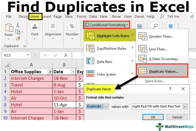
The first thing you have to do is highlight current duplicates in the selected Excel range. In this case, you have to follow the right steps. To implement this method, you have to follow these steps:
- First, select the data range on Excel that consists of the duplicate value. Make sure you don’t select the entire worksheet.
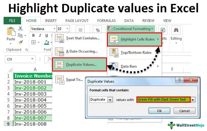
- Now, you have to click on the conditional formatting option under the ‘style’ menu of your Home tab. You can find ‘highlight cell rules’ there. You have to select the duplicate value here.
- The ‘duplicate values’ dialog box will be opened here. Now, you can choose the type of formatting as per your requirement. You can highlight the cell or the box with different colors.
- Next, you have to select the ‘light red fill with dark red text’ option and then click on OK. By doing this, you can highlight the value that is appearing more than once in a selected Excel range. The range will be highlighted after doing the process.
It’s very easy to implement. Still, you have to be careful here. You have to keep in mind that the conditional formatting feature can only highlight the duplicate values including the first occurrence.
2. Highlight Future Duplicates in the Selected Range
When it comes to how to highlight duplicates in Excel, many people ignore some crucial things. In this case, highlighting future duplicates in the selected range is also essential. If you follow this method, it will be very useful in the future. Let’s find out how to process it:
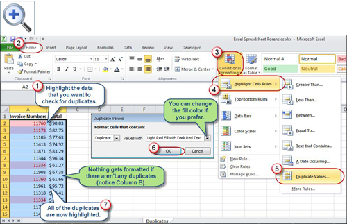
- First, select column A as you have to check if there’s any duplicate value entered in the list.
- Now, go to the Home tab and you have to click on the ‘conditional formatting’ drop-down under the ‘style’ option. Here, locate the ‘highlight cell rules’ and select the ‘duplicate values’ option.
- Next, you have to select a suitable color you want to use in the duplicate value cell. After selecting the color, you have to click on the ‘Ok’ option.
- Here, you can check the duplicate values on the selected column. For example, if you are choosing the yellow color, you can find one or more than one cell highlighted with yellow.
Alternatively, you can select the entire worksheet and follow the same instructions to get the result. It’s good if you have to handle a big invoice or project. However, there’s some difference between selecting the worksheet and only one column. In this case, you have to double-check everything before the implementation.
3. Remove Duplicates From the Selected Range
Nobody wants duplicate values in most cases. If you have the same intention, it’s easy to remove the value. Well, you have to follow some easy steps in this case. That’s why we are sharing how to remove duplicates from the selected range in the following guide:
- First, select the data range of duplicates
- Now, go to the ‘data tools’ group on the Data tab and select the ‘remove duplicates’ option.
- Here, you can see the ‘remove duplicates’ dialog box appeared. You have to check if there’s a selected box under the column.
- Next, you have to select the ‘my data has headers’ checkbox and then click on the ‘Ok’ option
- Well, the duplicate value is removed from your worksheet. Here, a message will appear where it will show the numbers of deleted duplicates from the column.
- Now, you can get only unique data in column A as all duplicates are removed.
Before you follow the steps while removing duplicates, you have to be careful. In this case, make sure you select the correct range where the duplicates are highlighted. That’s why highlighting the value is essential. On the other hand, you have to choose the correct column header as well. So, you can select the right formatting style.
Conclusion
Finally, you know how to highlight duplicates in Excel. We have shared the best ways to deal with this issue. Still, if you can’t solve anything, you can do some research on the internet. There are some tutorial videos and articles available. On the other hand, you can also contact an expert.
FAQs
Q: How do you select all duplicates in Excel?
If you want to select all duplicates in Excel, first you have to filter them and click on any filtered cell. It will help you select and then press ‘Ctrl+A’. If you want to select duplicate records without column headers, press Ctrl+Shift+End.
Q: How do I identify duplicates in Excel?
To identify duplicates in Excel, you have to select the cells you want to check and go to Conditional Formatting under the Home section.
Q: How do you highlight duplicates in sheets?
There are several steps you have to follow to highlight duplicates in sheets including highlighting the data, entering the custom duplicate formula, and more.
Q: How do you highlight duplicates in two columns in Excel?
To highlight duplicates in two columns in Excel, you have to select the data area and click on the Data tab. Then, select the Highlight Duplicate option and select ‘Set’.